Large Language Models (LLMs): a hitchhiker's guide to their galaxy (for newbies like me)

Large Language Models (LLMs) are revolutionizing how we interact with technology. As a software developer at lastminute.com, recently I started to use copilot during my daily job. In the last weeks I also attended the "Generative AI with Large Language Models" course to understand how LLMs work, and how to integrate them into my daily workflow, maximizing their benefits while avoiding pitfalls.

Recently, I've encountered situations where developers blindly copy-pasted code generated by LLMs without validation or code review, resulting in erroneous or nonsensical implementations. This is why I decided that I needed to understand how LLM works to better leverage their capabilities (and avoid mistakes like the one mentioned). This article serves as a structured reference of what I’ve learned so far, which I can revisit periodically and extend (similar to what I did for DDD some time ago).

The Evolution of LLMs

Before LLMs, text generation relied on Recurrent Neural Networks (RNNs). While these models improved sequential text generation, they struggled with long-term dependencies and training inefficiencies.

The game-changer came in 2017 with the paper "Attention Is All You Need" (Vaswani et al., 2017 [1]), which introduced Transformers. These models leveraged self-attention mechanisms to process input sequences in parallel, drastically improving efficiency and effectiveness.

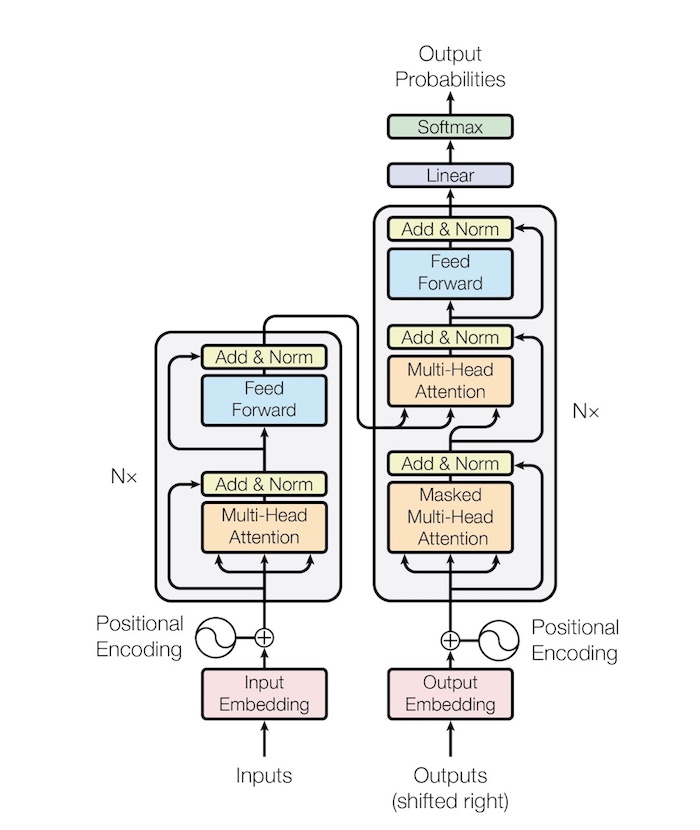
Transformer

Transformers consist of an encoder-decoder architecture:

• Encoder: processes the input sequence, generating contextualized embeddings. Each encoder layer consists of self-attention and feed-forward networks. The encoder is designed to understand and capture the relationships between words, producing an enriched representation of the input.
• Decoder: Generates the output sequence using encoded representations of the inputs using embeddings (like encoders) and previous outputs. The decoder attends to both its own previously generated tokens and the encoded input sequence, allowing for conditioned text generation.

Architecture Overview

Below you can see an illustration of the Transformer architecture (fromt the "attention is all you need" paper linked above):

Embeddings

Embeddings are dense vector representations of words or tokens that encode their semantic meaning. Each token in a sequence is mapped to a high-dimensional vector, capturing various linguistic relationships such as synonymy, analogy, and topic similarity.

For example, words that are semantically similar or contextually related tend to have similar embeddings. This is crucial for understanding language structures, as the embedding space captures these relationships and allows the model to make connections between words in different contexts.

In the Transformer architecture, the embeddings serve as the initial representation of the tokens before they are processed by the self-attention mechanism. These embeddings are often combined with the positional encodings, which provide the model with information about the position of each token within the sequence.

Together, embeddings and positional encodings enable the Transformer to process sequences in parallel while retaining both semantic meaning and the order of tokens.

Positional Encoding

As I said a few lines above, since the Transformers architecture is able to process words in parallel, positional encoding is used to retain the sequential order of tokens in a sequence. Without this encoding, the model would treat all tokens independently of their position in the sequence. The positional encoding is added to the token embeddings to provide the model with information about the position of each one of them in the sequence.

Position encoding is calculated using sinusoidal functions as reported in the paper "Attention Is All You Need" (Vaswani et al., 2017 [1]) in the "Positional Encoding" section. This choice guarantees that the positional encodings have a diverse set of frequencies (for long sequence length).

Self attention

Self-attention is the mechanism used in Transformer that enables each token in an input sequence to interact with every other token, allowing the model to learn dependencies between tokens, regardless of their position in the sequence.

In self-attention, each token in the input sequence is transformed into three components: query (Q), key (K), and value (V). These components are derived from the input embeddings by multiplying them by learnable weight matrices. Learnable weight matrices are parameters in the model that are adjusted during training to optimize the model's ability to map the input tokens to meaningful query, key, and value representations. These matrices are learned based on the data the model is exposed to, enabling the model to adapt its attention mechanism.

So going into the details of each component [2]:

• Query (Q): Represents the token that seeks information from other tokens.
• Key (K): Represents the characteristics of each word.
• Value (V): Represents the actual information of each word, like its meaning in the context of the sentence.

The core of self-attention involves computing a score to determine how much attention one token should give to another. This score is calculated by taking the dot product of the query and key vectors for each pair of tokens. These scores are then scaled by dividing by $(\sqrt{d_k})$ (where $(d_k)$ is the dimension of the key vector). This scaling helps to prevent the scores from becoming too large, which could lead to very small gradients during backpropagation, making learning difficult.

After scaling, the scores are passed through a softmax function, which normalizes them into a probability distribution. The attention scores represent attention patterns, which describe the model’s strategy for deciding how much focus (or attention) each token should give to other tokens. Different attention patterns help the model learn relationships in various ways, such as identifying direct associations or more abstract connections between tokens.

The weighted sum of the value vectors, based on the attention scores, gives the output for each token. This output is a mixture of all tokens in the sequence, weighted by how much attention each token should give to the others.

Mathematically, the self-attention operation can be represented as:

$$\text{Attention}(Q, K, V) = \text{softmax}\left(\frac{QK^T}{\sqrt{d_k}}\right)V$$

Where:

• $Q$, $K$, and $V$ are the query, key, and value matrices, respectively.
• $d_k$ is the dimension of the key vector (used for scaling).

Transformers use a multi-head self-attention mechanism, which splits the queries, keys, and values into multiple smaller "heads." Each head learns a different attention pattern, enabling the model to capture a variety of relationships simultaneously. The outputs of these multiple heads are then concatenated and projected back into the original embedding dimensional space though concatenation.

For example:

• One head might capture grammatical relationships (e.g., subject-verb agreement).
• Another head might focus on semantic similarity (e.g., synonyms in different contexts).
• A third head could handle long-range dependencies (e.g., connecting a pronoun with its antecedent in a long sentence).

Mathematically, multi-head attention is expressed as:

$$\text{MultiHead}(Q, K, V) = \text{Concat}(\text{head}_1, ..., \text{head}_h) W^O$$

where each attention head is computed as:

$$\text{head}_i = \text{Attention}(QW_i^Q, KW_i^K, VW_i^V)$$

Where:

• $W_i^Q$, $W_i^K$, and $W_i^V$ are learnable weight matrices for each attention head. They transform the input query, key, and value matrices for each head, enabling the model to learn different representations for different heads.
• $W^O$ is the weight matrix used to project the concatenated outputs of all the heads back into the original dimensional space.

Self-attention allows the model to process sequences in parallel and capture long-range dependencies efficiently, making it highly effective for tasks such as translation, text generation, and language modeling.

Transformer Model Types

The architecture described above is the general Transformer model. In practice, however, different tasks may only require part of this architecture, leading to the development of specialized Transformer variants. These include encoder-only, decoder-only, and encoder-decoder models, each optimized for specific tasks.

Encoder-Only Models

Encoder-only Transformers focus on understanding and extracting meaningful representations from text. These models process entire sequences bidirectionally, meaning they consider both past and future context simultaneously. They are particularly useful for tasks that require deep text comprehension.

The model consists only of the Transformer’s encoder stack. Each token embeddings attends to all other tokens in the sequence, allowing the model to capture dependencies between words.

These models are typically pretrained using Masked Language Modeling (MLM):

• During training, some tokens in the input sequence are randomly masked.
• The model learns to predict these missing tokens based on surrounding context.
• This forces the model to develop a deep contextual understanding.

Mathematically, given a sequence of tokens $X = (w_1, w_2, ..., w_n)$, the training objective is to maximize the probability of a masked token $w_i$ given its context:

$$P(w_i | w_1, ..., w_{i-1}, w_{i+1}, ..., w_n)$$

Some examples of encoder-only models are:

• BERT (Bidirectional Encoder Representations from Transformers) (Devlin, J., et al. 2018, [3]) – One of the most well-known encoder-only models, used for tasks like text classification, sentiment analysis, and question answering.
• ALBERT (Brown, T. B., et al. 2019, [4]) – A more efficient variant of BERT that reduces parameter size while maintaining performance.

Decoder-Only Models

Decoder-only Transformers are designed for generating text rather than understanding it. These models work in an autoregressive manner, predicting one token at a time based on the previous ones. They are widely used in applications that require free-form text generation.
The model consists only of the Transformer’s decoder stack. Unlike encoder-only models, which process input bidirectionally, decoder-only models are causal: they can only attend to past tokens.
During training, they use Causal Language Modeling (CLM):

• The model predicts the next token given all previous tokens in the sequence.
• It cannot see future words, ensuring it generates text sequentially like a human would.

Mathematically, given an input sequence $X = (w_1, w_2, ..., w_n)$, the training objective is to maximize the probability of the next token given the previous ones:

$$P(w_t | w_1, ..., w_{t-1})$$

This ensures the model learns to generate coherent and contextually relevant sequences.

Some examples of decoder-only models are:

• GPT (Generative Pre-trained Transformer) (Radford, A., et al. (2018). [5]), the most famous decoder-only model, used for tasks like chatbots, code generation, and creative writing.
• GPT-2 and GPT-3, more advanced versions of GPT, trained on massive datasets to improve generation quality.
• GPT-4, The latest version, capable of highly sophisticated text generation across diverse applications.

Encoder-Decoder Models

Encoder-decoder (or sequence-to-sequence) Transformers are designed for tasks that involve transforming one sequence into another, such as machine translation and text summarization. These models use both the encoder and decoder components of a Transformer.

The encoder processes the input sequence, converting it into a contextual representation. The decoder then generates the output sequence based on this encoded information.
Unlike decoder-only models, the decoder in encoder-decoder architectures attends to both previous output tokens and the entire encoded input.

These models are trained using Denoising Autoencoding, where parts of the input are randomly corrupted (e.g., some words are removed or shuffled), and the model learns to reconstruct the original sequence.

Mathematically, given a corrupted input sequence $X_{\text{corrupted}}$ and its original version $X$, the model learns to maximize the probability:

$$P(X | X_{\text{corrupted}})$$

This helps the model become robust in handling noisy or incomplete inputs.

Some examples of Encoder-Decoder models are:

• T5 (Text-to-Text Transfer Transformer) (Raffel, C., et al (2019). [6]), a highly flexible model where all tasks (translation, summarization, question-answering) are framed as text-to-text problems.
• BART (Bidirectional and Auto-Regressive Transformer), similar to T5, but with better handling of denoising tasks.
• mBART, a multilingual variant of BART, optimized for translation and multilingual text generation.

Training an LLM

Training a LLM is the process of teaching it to understand and generate human-like text by learning patterns from vast amounts of data. This training process enables the model to capture syntax, semantics, and contextual relationships within language, making it capable of performing tasks such as text completion, question answering, translation, and reasoning.

LLM training typically occurs in two main stages:

• Pretraining – The model learns general language patterns from a large corpus in an unsupervised manner.
• Fine-Tuning – The model is further refined on domain-specific tasks using supervised learning or reinforcement learning to improve its accuracy and usability.

Different training approaches, such as full pretraining, fine-tuning, retrieval-augmented generation (RAG), and prompt engineering, allow models to be tailored for specific applications while balancing efficiency and performance.

Full Pretraining

Pretraining is a crucial step in training large language models, where the model learns general language representations from vast amounts of text data. This phase is usually unsupervised or self-supervised, where the model attempts to predict certain aspects of the input data (such as masked words or the next word in a sequence) based on context. In this phase it is common to use techniques I discussed earlier like Masked Language Modeling (MLM) and Causal Language Modeling (CLM).

During pretraining, the model's parameters are optimized to minimize a loss function $L(\theta)$, where $\theta$ represents the model's parameters. This loss measures how far the model's predictions are from the actual target, which is defined by the specific pretraining task (again Masked Language Modeling (MLM) and Causal Language Modeling (CLM) that we saw before). The goal of pretraining is to adjust the model's weights such that the loss is minimized.

The optimization of the model’s parameters is achieved through backpropagation, a method that computes the gradient of the loss function with respect to each parameter in the model. The core idea of backpropagation is to propagate the error backward through the network, updating the weights in such a way as to reduce the overall error.

Mathematically, backpropagation is computed as the gradient of the loss function with respect to each weight $w_i$ in the model. The gradient $\nabla_w L$ for a weight $w_i$ is computed as:

$$\nabla_w L = \frac{\partial L}{\partial w_i}$$

This gradient tells us the direction in which the weight should be adjusted to minimize the loss. Once the gradient is computed, the weights are updated using gradient descent:

$$w_i \leftarrow w_i - \eta \nabla_w L$$

where $\eta$ is the learning rate, a hyperparameter that controls the size of the step taken in the direction of the gradient. In practice, the gradients are computed for all the weights in the model, and the parameters are updated iteratively to minimize the loss over many iterations or epochs. In practice, the gradients are computed for all the weights in the model, and the parameters are updated iteratively to minimize the loss over many iterations or epochs.

The effectiveness of backpropagation depends heavily on the gradient flow during training. If the gradients are too small (a phenomenon known as vanishing gradients), the model may not learn effectively. On the other hand, if the gradients are too large (a phenomenon known as exploding gradients), the model's weights can be updated in a chaotic manner, leading to unstable learning.

An example in the industry, apart from ai-focused companies, is BloombergGPT, a domain-specific pretrained model optimized for financial data analysis.

Fine-Tuning

Fine-tuning an existing model is more efficient than full pretraining. It involves modifying the weights of an already trained model to specialize it for a specific task. Instead of training from scratch, the model is initialized with pretrained parameters and then updated based on new labeled data.

Gradient updates during fine-tuning modify the model’s representations while retaining its general knowledge:

$$\theta' = \theta - \eta \nabla_{\theta} L$$

where $\theta$ are the model parameters, $\eta$ is the learning rate, and $L$ is the task-specific loss function.

Parameter-Efficient Fine-Tuning (PEFT)

PEFT techniques optimize training by adjusting only a subset of weights, preventing catastrophic forgetting (where new training data overwrites prior knowledge). This makes fine-tuning more computationally feasible.

LoRA (Low-Rank Adaptation)

LoRA injects low-rank matrices into pre-trained layers, reducing the number of trainable parameters while preserving the model’s capabilities. Instead of updating all weights, LoRA decomposes weight updates into two low-rank matrices $A$ and $B$:

$$\Delta W = A B^T$$

How does it works?

• The original model's weights $W$ remain frozen (unchanged).
• Instead of updating $W$, we train only the small matrices $A$ and $B$.
• During inference, the modified weights are computed as $W + \Delta W$.

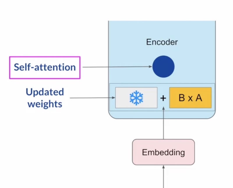
This significantly reduces memory and computational requirements for training.

Soft Prompts

Soft prompts replace traditional text-based prompts with learned embedding vectors, enabling lightweight adaptation without altering the model’s core parameters. These embeddings are optimized directly in the high-dimensional space the model operates in.

Enhancing using information in the contextual window

Enhancing LLMs with Contextual Information refers to the process of improving the performance and relevancean LLM by incorporating additional context beyond the input prompt.

Prompt Engineering

Prompt engineering is the practice of crafting input prompts to guide a language model’s responses effectively. By structuring the prompt in a specific way, users can influence how the model interprets and generates text. This technique is essential for maximizing the performance of LLMs without modifying their underlying parameters.

There are several key strategies in prompt engineering:

• Zero-shot learning: The model is given no prior examples and must generate a response based solely on its pre-trained knowledge. This is useful when testing the model’s ability to generalize to new tasks without explicit guidance.
• One-shot learning: The model is provided with a single example before making a prediction. This helps to slightly adjust its behavior by demonstrating the expected format or reasoning process.
• Few-shot learning: The model is given multiple examples to learn from before generating a response. By providing a small set of demonstrations, the model can better infer the intended task and produce more accurate or contextually appropriate outputs.

Retrieval-Augmented Generation (RAG)

Retrieval-Augmented Generation (RAG) is a hybrid approach that enhances LLMs by dynamically retrieving relevant external knowledge before generating a response. RAG integrates retrieval mechanisms to access up-to-date or domain-specific information, improving factual accuracy, reducing hallucinations, and enabling models to handle specialized queries more effectively without the need of fine tuning of full pretraining.

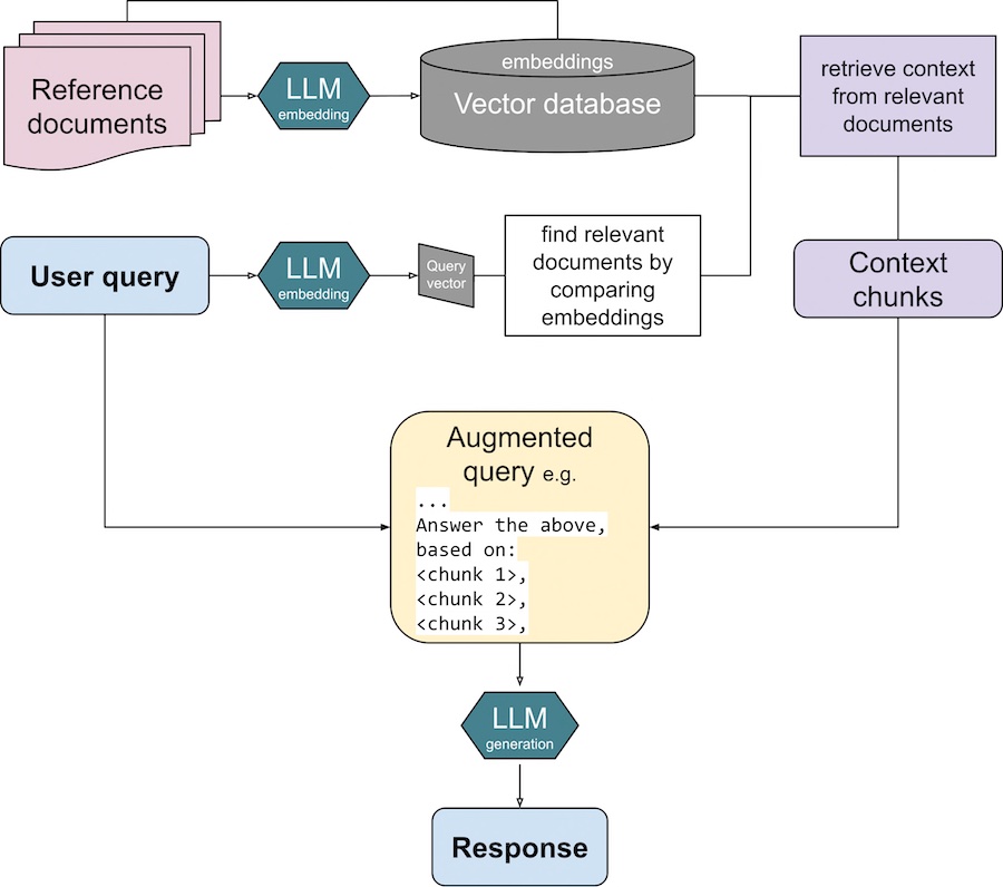
RAG consists of two main components:

• Retrieval: Given a user query, the system searches a knowledge source (e.g., a vector database) to find the most relevant documents, snippets, or embeddings.
• Generation: The retrieved information is incorporated into the model’s prompt and used to condition its response, ensuring that outputs are informed by external knowledge source.

At the core of RAG's retrieval step is similarity search in a vector space. Each document from the external source is represented as embedding $v$. The retrieval process is based on measuring the cosine similarity between the query vector $q$ and a candidate document vector $d$:

$$\text{sim}(q, d) = \frac{q \cdot d}{\|q\| \|d\|}$$

where:

• $q$ is the query vector (representing the user’s input)
• $d$ is a document vector (representing a knowledge snippet)
• $q \cdot d$ is the dot product between the vectors
• $\|q\|$ and $\|d\|$ are their respective magnitudes (norms)

The higher the similarity score, the more relevant the document is to the query. The system retrieves the top-k most relevant results before passing them into the prompt to the LLM for response generation.

RAG has some advantages over other traning techniques:

• allows models to access industry-specific data without requiring full retraining/fine tuning.
• reduced model size requirements: instead of embedding all knowledge in model weights, RAG enables efficient retrieval from external sources, making large-scale models more practical.

To perform the efficient retrieval described above, RAG relies on specialized vector databases, which index and store embeddings for fast similarity searches. Some popular options include:

• FAISS (Facebook AI Similarity Search): A high-performance library optimized for fast nearest neighbor searches in large-scale datasets.
• Chroma: A developer-friendly and easily integrable vector database designed for AI applications.
• Redis: Supports real-time querying and efficient indexing, making it a good choice for applications requiring low-latency responses.

Program-Aided Language (PAL)

PAL augments LLMs with external computation capabilities, allowing them to execute code snippets or run calculations instead of simply predicting text.

For example, instead of answering "What is 17 factorial?" using text generation, PAL enables the model to execute Python code:

import math
print(math.factorial(17))

This approach ensures accuracy in numerical and logical reasoning tasks.

Chain-of-Thought (CoT) Reasoning

Chain-of-Thought (CoT) is a technique that enables LLMs to break down complex reasoning tasks into intermediate steps. Instead of predicting an answer in a single step, the model explicitly generates a sequence of logical steps leading to the final answer.

CoT extends the model's response length, allowing it to articulate intermediate reasoning before arriving at a solution.
This is particularly effective for math problems, logic puzzles, and commonsense reasoning, where direct pattern matching is insufficient.
Here below an example of a task executed without and with CoT.

**Question:** *A farmer has 3 cows, 4 chickens, and 2 goats. How many legs do all the animals have in total?*  

**Without CoT:**  
*"The answer is 32."*  

**With CoT:**  
*"Cows have 4 legs each, so 3 × 4 = 12 legs. Chickens have 2 legs each, so 4 × 2 = 8 legs. 
Goats have 4 legs each, so 2 × 4 = 8 legs. The total number of legs is 12 + 8 + 8 = 28."*  

This structured reasoning approach reduces hallucinations and improves problem-solving accuracy.

ReAct (Reasoning + Action)

ReAct combines the techniques presented ealier with interactive decision-making. Unlike RAG, which retrieves external knowledge and stops, ReAct enables the model to take actions and refine its responses dynamically.

For example, a ReAct model could:

• Retrieve context using RAG.
• Generate a reasoning step using Chain-of-Thought.
• Execute external API calls to refine its output.

This makes it useful in autonomous agents and interactive AI applications.

Conclusion

In this article, I summarize the knowledge I’ve gained over the past few weeks of studying and taking courses on Large Language Models (LLMs). While these tools are undeniably powerful, they still require human creativity to guide them effectively.

That being said, it's clear that, when used thoughtfully, they can significantly accelerate workflows and improve your performance in ways we’ve never seen before.

Will we be replaced by an AGI (Artificial General Intelligence) in the future? It's probably still uncertain. Personally, I’m not a magician (yet 😅), so I don't know the answer. To be honest, it's already hard enough to know if I will be alive tomorrow. However, it’s both exciting and somewhat unsettling to witness how technology is advancing at a pace faster than society can keep up with. Will we be ready for such a monumental shift? I’m don't think so. For now let's embrace the productivity boost these tools provide. After all, we live one day at a time.

References

• [1] Vaswani et al., 2017, "Attention is all you need"
• [2] Understanding the Transformer Attention Mechanism
• [3] Devlin, J., et al. (2018), "BERT: Pre-training of Deep Bidirectional Transformers for Language Understanding. In Proceedings of NAACL-HLT 2019"
• [4] Brown, T. B., et al. (2019). Language Models are Few-Shot Learners. In Proceedings of NeurIPS 2020.
• [5] Radford, A., et al. (2018). Improving Language Understanding by Generative Pre-Training.
• [6] Raffel, C., Shazeer, N., Roberts, A., Lee, K., Narang, S., Matena, M., Zhou, Y., Li, W., & Liu, P. J. (2019). Exploring the limits of transfer learning with a unified text-to-text transformer.